
Investigating the Relative Uncertainty of the Degree of Urbanisations Output Classifications using Four Population Models, Nigeria
Abstract
Currently, the categorisation of the urban-rural continuum varies depending on national definitions — diminishing the effectiveness of international statistical comparison. The United Nations Sustainable Development Goals, for example, demands a universal measuring standard. The degree of urbanisation classification seeks to provide the solution. Effectively, the classification categorises the urban-rural continuum by 1 km2 gridded cells using population characteristics; instead of using localised spatial units or definitions. In various countries, however, inaccurate census data prevails. Where population data remains limited estimation models are used. The purpose of this report is to assess the relative uncertainty of the degree of urbanisation’s varying classification outputs — when inserting different population models into the tool for the same area. Specifically, the paper explores Nigeria in 2020. The population estimation models encompassed WorldPop Top-down Unconstrained, WorldPop Top-down Constrained, WorldPop Bottom-up and GHSL’s GHS-POP model. If the classification outputs vary greatly, the methodology — endorsed by the United Nations Statistical Commission — is ineffective for classifying countries using modelled datasets. To compare the classification outputs a classification analysis, entropy and binary comparison were used. These sensitivity analysis tests uncovered the WorldPop Top-down Unconstrained dataset was dissimilar compared with the other population estimation models. The results were later presented to the European Commission. For future research, testing and comparing different countries — with opposing population patterns — to Nigeria holds importance.
Introduction
Across the globe national definitions categorising the urban-rural continuum vary — reducing the capacity to undertake international statistical comparison. The degree of urbanisation classification, endorsed by the United Nations Statistical Commission, offers a universal methodology for comparison (Dijkstra et al., 2021). Eurostat (2021) illustrates the methodology classifies the urban-rural continuum into equal sized 1 km2 gridded cells; instead of employing localised spatial units. At the first level the degree of urbanisation classifies the gridded cells based on the populations size, density and contiguity. Eurostat (2021) defines the first level’s three distinct classifications as urban centres, urban clusters and rural grid cells. Through classifying the urban-rural continuum into equal gridded cells the capacity to measure the United Nations Sustainable Development Goals is enhanced. Critically, classifying for goals requiring specific urban or rural indicators — including access to public transport — improves policymaking (Dijkstra et al., 2022). Following the degree of urbanisation’s emergence as a methodology to undertake international statistical comparison, the European Commission (2020a) has demanded further investigation.
One key challenge the European Commission (2020a) identified comprised of accounting for the absence of correct geo-coded censuses or population registers. Currently, the time delay amid resource-poor countries data collection and publication lessens censuses robustness; whilst corruption prevails where population is linked with resource allocation (Wardrop et al., 2018). Where the unavailability of correct datasets exists, Eurostat (2021) recommends creating a disaggregation grid. Eurostat (2021) instructs disaggregation grids are formed using a combination of population models and land use data. The population models, however, vary in structure and covariates (Wardrop et al., 2018). Effectively, for the degree of urbanisation to produce results for international statistical comparison — the methodology necessitates producing uniform results regardless of population model inputted (Dijkstra et al., 2021). The reports’ purpose, therefore, is to employ a sensitivity analysis towards uncovering the relative uncertainty of inserting different population models into the degree of urbanisation methodology. If the outputs vary greatly, the tool is ineffective for classifying countries using modelled datasets — addressing a challenge outlined by European Commission (2020a).
To start, the degree of urbanisation alongside strategy to address the challenge — namely exploring variations in classification outputs using different population models — have been introduced and justified. Following this, the methods section first describes the data selection and characteristics; then establishes the workflow using GIS; before finishing with the methods of sensitivity analysis. The results section precedes, comprising of the appropriate tables and maps. Subsequently, the discussion seeks to explore and compare the metrics alongside the classification outputs. Finally, the conclusion seeks to synthesise the findings and present future research topics.
Methods
Data Selection
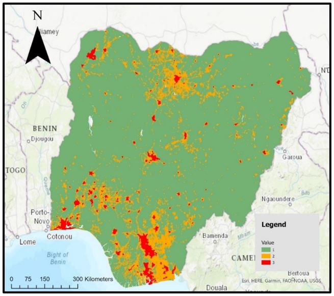
Nigeria was selected for investigation owing to the diverse range of existing population models and real-world application. Nigeria’s last census, conducted in 2006, was deemed unacceptable by the countries National Population Commission (Serra and Jerven, 2021). The predominant invalidating factors encompassed widespread over enumeration and settlement omission — population models thus remain Nigeria’s sole option for applying the degree of urbanisation (Serra and Jerven, 2021). Effectively, the real-world application of utilising population models frames Nigeria as appropriate towards attaining the research aims. Likewise, an abundance of population models enable comparison of classification output (Bondarenko et al., 2020; Schiavina et al., 2022). These models illustrate Nigeria’s dense populations surrounding Lagos on the coast and Kano in the north; whilst large rural expanses prevail in the far east and west (Bondarenko et al., 2020).
Within the investigation 4 population models for the year 2020 were chosen to process through the degree of urbanisation workflow and thereafter analyse the output. The population models encompassed WorldPop’s Top-down Unconstrained dataset, Top-down Constrained dataset and Bottom-up dataset (Bondarenko et al., 2020; WorldPop, 2018a; WorldPop and National Population Commission of Nigeria, 2021); with the addition of the GHS Population Grid (Schiavina et al., 2022). For later comparison, a mixture of constrained and unconstrained datasets was selected. Constrained models limit population to areas with building presence; instead, unconstrained models allocate population ubiquitously (Thomson et al., 2021).
For each population model the corresponding settlement datasets was also required to implement the 50% Built-up in Urban Cluster rule. The 50% rule was incorporated owing to the European Commission (2020b) expressing the action mitigates the issue of allocating populations to low density urban sprawl — through producing urban centres based on cells with a density of 1,500 and are 50% permanently built-up. Preliminary testing illustrated implementing the 50% rule limited most of the urban centre’s size, though the individual centres were not completely omitted. Below is a table highlighting the differences amid the population estimation models and corresponding underlying settlement datasets.
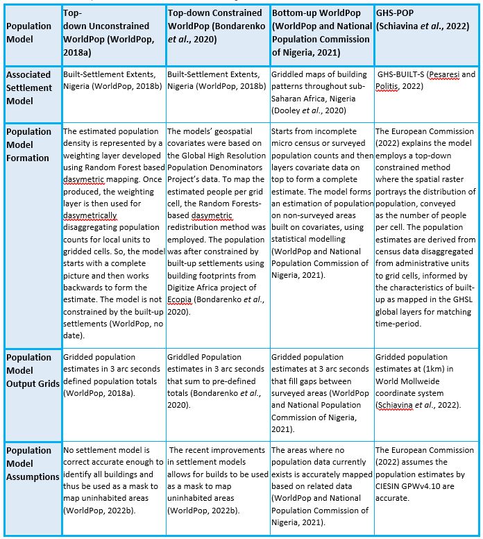
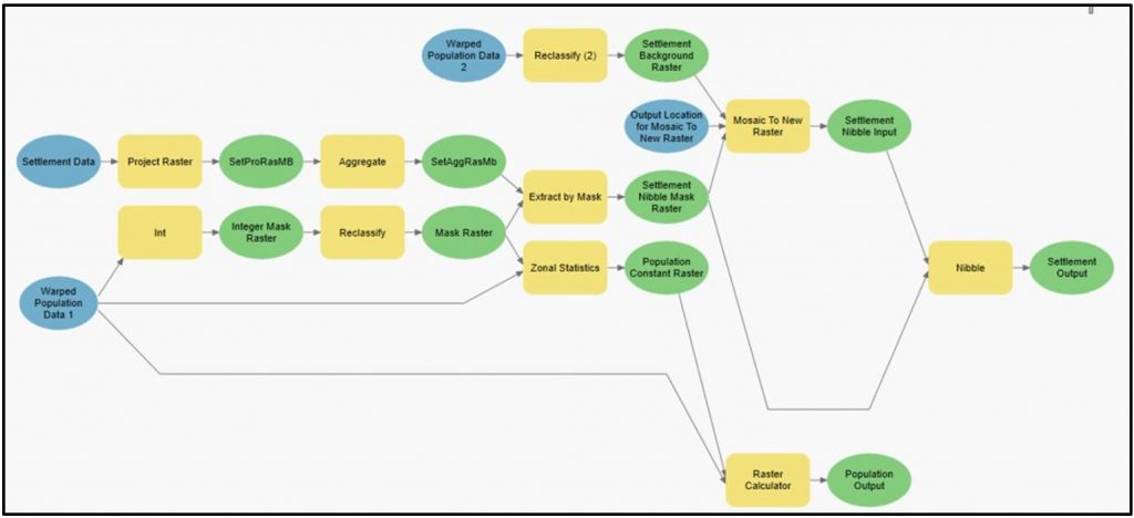
Figure 1 displays a model created using ArcGIS Pro Model Builder illustrating the workflow employed. Unless using a GHSL standalone tool, the complete workflow displayed used ArcGIS Pro Version 2.9.3. Before stating the workflow illustrated within figure 1, however, implementing the European Commission’s (2021) GHS-POPWARP standalone tool must transpire. The specific details of processing pane input information are found in the appendix. The European Commission (2021) express the purpose of the GHS-POPWARP standalone tool is reprojecting the population models from a geographic coordinate system to a projected coordinate system — namely Mollweide — whilst maintaining volume. Owing to the degree of urbanisation’s stipulation for equal gridded cells, the later used GHS-DUG standalone tool, produced by the European Commission (2020b), only supports projected coordinate systems. So, utilising the GHS-POPWARP standalone reprojecting function stood necessary. Through experimentation, the standalone versions for all GHSL tools were processed quicker, compared with ArcGIS Pro versions, thus were preferred.
The following section entailed creating a ‘Mask Raster’ to function as a consistent mask, overlapping unwanted features for both population and settlement models (Esri, no datea). As the figure 1 illustrates, ‘Warped Population Data 1’ processed through the Int (Spatial Analyst) and Reclassify (Spatial Analyst) geoprocessing tools. The specific inputs into the geoprocessing pane are found in the appendix. The Int (spatial analyst) tool held necessity as the Reclassify tool only supports integers; thereafter the Reclassify (spatial analyst) transformed ‘Integer Mask Raster’ into a singular value (Esri, no datec).
To ensure the population models were comparable for later statistical analysis, attaining equal population counts for each population model ensued. The process adjusted population counts to the UNPD estimates for 2020 (United Nations Population Division, 2022), using the equation ‘popi* UNPD_pop/country_tot_popi)’ (Sorichetta et al., 2015). Within the equation popi is the estimated population raster for the year, UNPD_pop is a constant raster representing the 2020 UNPD estimates, and country_tot_popi is a constant raster representing the total pop for the year (Sorichetta et al., 2015). To achieve adjusted population counts, figure 1 demonstrates ‘Warped Population Data 1’ processed through Zonal Statistics (Spatial Analyst) and the Raster Calculator (Spatial Analyst). The Zonal Statistics (Spatial Analyst) produced the ‘Population Constant Raster’ using the sum function; whilst the Raster Calculator (Spatial Analyst) used the equation to produce the adjusted population counts. An optional check, found in the appendix, uses zonal stats to sum each pixel of the new ‘Population Output’ to ensure the total equals the UNPD 2020 estimate.
The final stage presented in figure 1 depicts the ‘Settlement Data’ transforming from a categorical to continuous data type and the subsequent nibbling to eliminate inconsistent pixels. The European Commission (2020b) states the GHS-DUG standalone tool only supports continuous datasets, so the categorical WorldPop ‘Settlement Data’ requires a data type transformation. The transformation entailed using Project Raster (Data Management) to 100-meter grid cells, then applying Aggregate (Spatial Analyst) to 1000-meter grid cells.
Following the data type transformation, the preparation for nibbling ensued. Nibble’s (Spatial Analyst) functioned to reduce inconsistencies surrounding the coastline where differing settlement models may allocate additional buildings. Effectively, where discrepancies exist the settlement model’s structure is unable to clarify whether 0’s are no data, are no people, or are no buildings. To resolve the issue, Nibble (Spatial Analyst) produces raster’s where 0 equates to no buildings (Esri, no datab). To complete nibbling, a settlement mask was required (Esri, no datab). Applying Extract by Mask (Spatial Analyst), employing the ‘Raster Mask’ derived from population data, ensured the ‘Settlement Nibble Mask Raster’ possessed a corresponding extent with the ‘Population Output’ — in preparation for the European Commission’s (2020b) GHS-DUG standalone tool.
Similarly, for the Nibble (Spatial Analyst) to perform the pixels of ‘Settlement Nibble Input’ necessitated a value where no data corresponded with the extent of ‘Warped Population Data 2’. Effectively, the now assigned values of ‘Settlement Nibble Input’ are nibbled to the closest value where no data persists in the ‘Settlement Nibble Mask Raster’ (Esri, no datab). Ultimately, producing raster’s where the extents are uniform with ‘Warped Population Data 2’. For clarification, the ‘Warped Population Data 2’ is the same raster as ‘Warped Population Data 1’. As figure 1 illustrates, ‘Warped Population Data 2’ uses Reclassify (Spatial Analyst) to allocate a single value greater than all ‘Settlement Nibble Mask Raster’ values. The Mosaic to New Raster (Data Management) tool then combines the created ‘Settlement Background Raster’ with the ‘Settlement Nibble Mask Raster’. So, the formed ‘Settlement Nibble Input’ now possesses values — corresponding to the extent of ‘Warped Population Data 2’ — where no data persists in the ‘Settlement Nibble Mask Raster’. The Nibble (Spatial Analyst) thereafter produced the ‘Settlement Output’; where the raster’s no data values indicate absence of buildings and possesses the same extent as the ‘Population Output’.
After completing the workflow outlined in figure 1, the ‘Population Output’ and ‘Settlement Output’ files are prepared for the GHS-DUG standalone tool. Specific details of the input information for the GHS-DUG standalone tools exists within the Appendix. The European Commission’s (2020b) GHS-DUG standalone tool creates a settlement classification gridded raster that maps the three distinct degree of urbanisation classifications. Eurostat (2021) details the threshold for each classification:
- Urban Centre – a dense cluster of continuous 1km2 grid cells, employing a 4-point contiguity that excludes diagonals, containing a population density of minimum 1,500 inhabitants per 1km2. The collective population of the urban centre must reach 50,000 residents. Breaks in the cluster are filled if lesser than 15km2; whilst continuous cells that are minimum 50% built-up may be included. Urban centre cells are classified as ‘3’ in red.
- Urban Cluster – A moderate density cluster consisting of continuous 1km2 grid cells, employing an eight-point contiguity that includes diagonals, containing a population density of at least 300 inhabitants per 1 km2. The collective population of the urban cluster must reach 5,000 residents. The urban centre cells are removed from the urban cluster. Urban cluster cells are classified as ‘2’ in orange.
- Rural Grid Cells – Mostly low-density cells that are not classified as urban centres or as urban clusters. Rural grid cells are classified as ‘1’ in green.
In effect, the outcome of applying the GHS-DUG standalone tool for all four cases of population model type produces four output rasters detailing the three classifications. Before analysis, the output rasters clipping to matching extents, owing to the outputs from the European Commission (2022b) GHS-DUG standalone tool appearing in tile form). The Clip Raster (Data Management) tool used the ‘Mask Raster’ — derived from the Top-down Unconstrained population model — upon all outputs to match the extents to Nigeria’s boundary. Within the geoprocessing tool pane, keep ‘maintain clipping extent’ unticked and snap to the GHS-DUG output. The Top-down Unconstrained population model’s mask was selected as the raster holds the largest area. The produced rasters are now prepared for statistical analysis.
Statistical Analysis
Classification Statistics
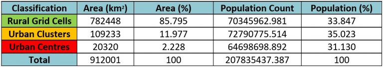
The first investigation comprised of a statistical analysis focusing on the area and populations of each distinct classification. The method entailed applying Zonal Statistics as Table (Spatial Analyst) to sum each output of the GHS-DUG tool; subsequently, exporting the table to excel. Calculating the percentages and standard deviation for each table ensued. Ultimately, the classification statistics comprised of the real area and population of each GHS-DUG output, with the associated percentages and standard deviation. Similar approaches were performed in related papers (Bueno et al., 2019; Dijkstra et al., 2021).
Entropy
The purpose applying entropy was to understand the frequency of pixel value change across the 4 GHS-DUG outputs. Doing so, held significance to determine variation in classification type. Entropy proved appropriate as the concept measures the frequency difference of a phenomenon across a range (Mohajeri et al., 2013). The entropy output map — supplied by Dr Maksym Bondarenko of WorldPop — displayed the frequency of change, amid all 4 output rasters. Once obtained, the map was converted into an integer using the Int (Spatial Analyst) and Raster Calculator (Spatial Analyst) geoprocessing tools. The raster’s associated table was after exported to excel where associated percentages were calculated.
Binary Comparison
The final analysis sought to uncover the degree of change amid jumping pixel values. The previous approaching utilising entropy only displays whether the pixel has jumped, not the number of jumps. If one GHS-DUG output pixel jumped from urban centre to urban cluster and the remaining rasters stayed as urban centre; whilst a different pixel jumped from urban centre to rural grid cell with the remaining pixels staying as urban centre — entropy would present the same score (Mohajeri et al., 2013). Uncovering the extent of change holds importance, since greater discrepancies indicate greater uncertainty in the degree of urbanisations methodology. Binary Comparison compensates for the lack of information entropy provides — through displaying the degree of jumping as percentages (Sorichetta et al., 2011).
The method encompassed dividing three of the GHS-DUG output rasters individually by the GHS-POP GHS-DUG output raster, using the Raster Calculator (Spatial Analyst). GHS-POP was selected as the standard for comparison as the European Commission (2022) produces the GHSL products and is the baseline (European Commission, 2022).
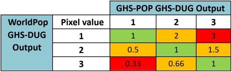
After dividing each GHS-DUG output by GHS-POP, the three produced rasters were individually multiplied by 100 and turned into an integer; applying the Raster Calculator (Spatial Analyst) and Int (Spatial Analyst) tools respectively (Sorichetta et al., 2011). The three raster’s associated tables were thus exported to excel and calculating percentages based on extent of pixel jumps followed. Table 2 illustrates the output values of binary comparison — where green values indicate the pixels are the same, orange indicates a jump of 1 and red indicates the pixel jumped twice.
Results
GHS-DUG Output
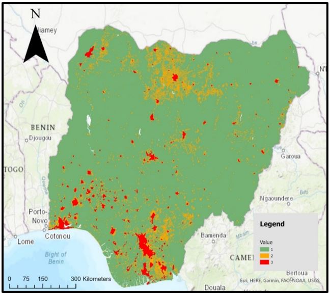
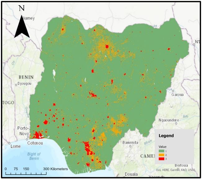
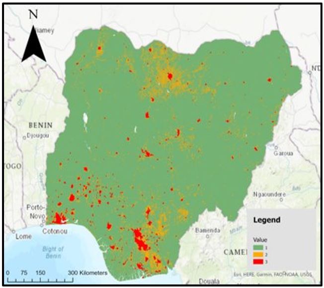
Figures 2, 3, 4 and 5 illustrate the final clipped output from the GHS-DUG tool. Visually, the figures show rasters that possess relatively similar spatial patterns. The red urban centres appear in the same areas; whilst the green rural grid cells are allocated uniformly. The largest discrepancy is amid the orange urban clusters. Figure 2, for example, displays a greater frequency of orange urban clusters compared with the remaining three figures. Overall, however, the GHS-DUG outputs present rasters with similar spatial patterns.
Classification Statistics
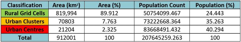
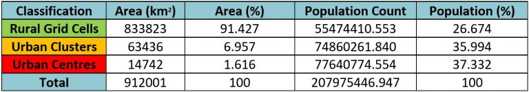
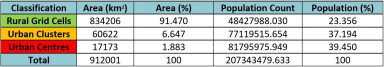
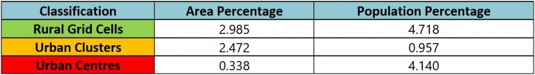
Comparable to the rasters produced from the GHS-DUG standalone tool, the classification statistics produced similar results for each GHS-DUG output. The first point of interest shown in the tables below, however, concerns the WorldPop Top-down Unconstrained population in rural grid cells. The percentage is approximately 9% higher compared with the remaining tables. Likewise, table 3 shows WorldPop Top-down Unconstrained rural grid cells area are approximately 5% smaller. So, the WorldPop Top-down Unconstrained GHS-DUG output comprises of a larger rural population within a smaller area. The remaining GHS-DUG outputs area and population are highly similar. WorldPop bottom-up and GHS-POP’s area are particularly alike. The two standard deviations that are relatively high are rural grid cell and urban centre populations — appearing at 4.718 and 4.140 respectively. In contrast, the urban centre area and urban cluster population both possess a standard deviation lower than 1, indicating small variation surrounding the mean. Upon reflection, although the classification statistics are largely similar, the WorldPop Top-down Unconstrained presents the greatest comparative difference; whilst rural and urban centre’s standard deviation produced the greatest variation.
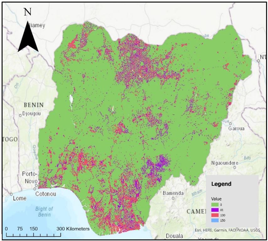
Entropy
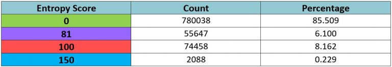
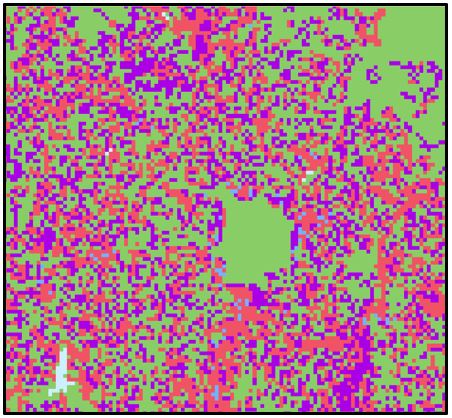
Figure 6 displays the entropy map with the associated values of pixel change. Where the score is 0 all the rasters remained the same, 81 indicated a single difference amid the rasters, 100 indicated 2 rasters were different, and 150 indicates 3 rasters are different. The entropy scores illustrate most pixels did not change value — namely, 85.509%. Many of these pixels are displayed in rural grid cells. The largest urban centres, however, are also displayed in green. Kano in the north, shown in figure 8, presents a green centre surrounded by pixels that did change. In general, the urban clusters surrounding urban centres changed classification the most. Very few pixels — only 0.229% — were classified differently in each of the GHS-DUG outputs. The largest group of these pixels scoring 150 are displayed in figure 8. The remaining pixels that scored 150 were diffuse individual pixels. Entropy thus demonstrated pixels characterised as an urban centre or rural grid cell were similar across the different GHS-DUG outputs; instead, the urban clusters experienced the greatest variation.
Binary Comparison
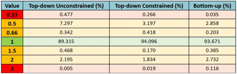
Table 9 illustrates the extent of pixel jumps in comparison to the GHS-POP GHS-DUG output. Alike to the statistical comparison, the WorldPop Top-down Unconstrained GHS-DUG output proved comparatively different. The non-jumping pixels were approximately 4% lower compared to the remaining models — indicating a higher number of jumps overall. Similarly, the 0.33 and 0.5 values for Top-down Unconstrained were comparatively higher, again indicating greater variation. According to the table 2, a high 0.33 and 0.5 value indicates the Top-down Unconstrained possessed a greater proportion of urban centres and urban clusters pixels jumping compared to GHS-POP’s rural areas. The Top-down constrained and Bottom-up GHS-DUG outputs instead possessed a similar number of jumps in comparison to the GHS-POP GHS-DUG output. Overall, however, a large percentage — between 89.315% and 94.096% — of pixels did not jump. So, despite the Top-down Unconstrained pixels jumping more often, generally the pixels were jumped infrequently.
Discussion
The Dissimilarity of WorldPop Top-down Unconstrained
Across each analysis method, the Top-down Unconstrained GHS-DUG output proved the most distinct compared with other population models. Among the rural grid cell classification, for example, the Top-down Unconstrained model allocated the greatest percentage of population and least amount of area. The cause of the phenomenon is likely due to the population estimation model’s structure. Unconstrained population model’s do not limit population to building footprints — so may allocate population where constrained population models exclude population — causing an overestimation of miscellaneous population in rural areas (Thomson et al., 2021). The standard deviation metrics reflected the population variation amid of unconstrained and constrained models. When the top-down unconstrained dataset was removed, the rural grid cell standard deviation decreased from 4.718 to 1.381. Likewise, the urban centre standard deviation decreased from 4.140 to 1.526. Evidently, the Top-down Unconstrained GHS-DUG output is the primary cause of variation in population.
The structure of the Top-down Unconstrained population model is likely also the cause of the lower rural grid cell area allocation. Within the constrained population rasters, the no data pixels indicated where the building footprints were. In the WorldPop Top-down Constrained GHS-DUG output 366,030 km2 counted as no data; whilst in the WorldPop Bottom-up raster 373,104 km2 was counted as no data. In effect, including the building footprints constraint increased the pixels allocated too rural. The binary comparison — also focusing on pixel area — similarly demonstrated the Top-down Unconstrained GHS-DUG output produced a greater frequency of pixel jumps. Beyond this study, future work focusing on a population-based binary comparison may present a further pronounced difference. After comparing the different GHS-DUG outputs the Top-down Unconstrained population model was, therefore, the most significantly distinct.
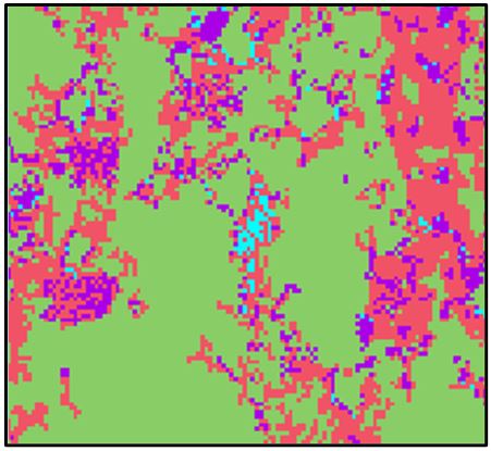
The Degree of Urbanisations Effect on Urban Clusters
The urban cluster classification across the 4 GHS-DUG outputs produced the greatest frequency of inconsistencies. The entropy clearly demonstrated the phenomenon — where the greatest number of changing pixels surrounded major urban centres. Significantly, figure 7 highlights an area surrounding the major urban centre of Ibadan, where the group of pixels changed with each GHS-DUG output. The claim Ibadan’s urban-rural continuum caused the group in Figure 7, however, is an assumption. Diffuse rivers in the location may also cause the discrepancies between GHS-DUG outputs. Nonetheless, the binary comparison demonstrated urban clusters posed greater inconstancies amid GHS-DUG output. Table 9 illustrated very rarely do pixels jump from a rural grid cell to urban centre from a WorldPop to GHSL population model. Instead, the pixels are predominantly jumping once, from urban centre to urban cluster or rural grid cell to urban cluster. Although the results indicate greater variation in urban clusters, ultimately the result is positive for the European Commission. Rather than allocating the pixels to the opposite classification, the degree of urbanisation predominantly allocates the pixels differently by one. Though positive, a focus for European Commission to improve the degree of urbanisation tool may entail producing greater precision when allocating urban clusters.
Conclusion
The report sought to address the challenge of consistency when using population estimation models within the degree of urbanisation classification — outlined by the European Commission (2020a). Assessing the relative uncertainty of inputting varying population estimation models revealed generally the classification outputs were similar. Despite the general precision, the population estimation model displaying the greatest variation was the WorldPop Top-down Unconstrained dataset. A suggestion for policymakers and the European Commission may, therefore, arise as only applying constrained population estimate models. Though the Top-down Unconstrained population model proved the most inconsistent comparatively, overall few pixels changed amid the 4 models. The green expanse in figure 6, representing 85.509% of pixels maintaining the same classification across all models, illustrates the similarities. Without comparing these results with alternate countries, however, it stands impossible to comprehend whether 85.509% is high-quality. Equally, Nigeria may befall as an outlier — with other countries possessing greater variation. Appropriate countries for future research include Namibia or the Dominican Republic. Both countries possess dissimilar population characteristics to Nigeria; whilst also possess suitable population estimation models (WorldPop, 2022a). As the tests completed in the report are reproducible, the future research is possible.
References
- Bondarenko, M., Kerr D., Sorichetta, A., and Tatem, A.J. (2020) ‘Census/projection-disaggregated gridded population datasets for 51 countries across sub-Saharan Africa in 2020 using building footprints. WorldPop, University of Southampton, UK’. Available at: https://hub.worldpop.org/geodata/summary?id=49654 (Accessed: 28 June 2022).
- Bueno, M.D.C.D. and Lima, R.N.D.S. (2019) ‘The degree of urbanisation in Brazil’, Regional Statistics, 9(1), pp. 72-84.
- Dooley, C. A., Boo, G., Leasure, D.R. and Tatem, A.J. (2020) ‘Gridded maps of building patterns throughout sub-Saharan Africa, version 1.1. WorldPop, University of Southampton. Source of building footprints: Ecopia Vector Maps Powered by Maxar Satellite Imagery (C) 2020’. Available at: https://wopr.worldpop.org/?NGA/Buildings/v1.1 (Accessed: 23 June 2022).
- Dijkstra, L., Florczyk, A.J., Freire, S., Kemper, T., Melchiorri, M., Pesaresi, M., Schiavina, M. (2021) ‘Applying the Degree of Urbanisation to the globe: A new harmonised definition reveals a different picture of global urbanisation’, Journal of Urban Economics, 125, pp. 1-27.
- Dijkstra, L., Galic, A. and Brandmüller. (2022) ‘Measuring Sustainable Development Goals in cities, towns and rural areas: The new Degree of Urbanisation’, Statistical Journal of the IAOS, 38(2), pp. 549-559.
- Esri (no date) Mask Features. Available at: https://pro.arcgis.com/en/pro-app/latest/help/mapping/layer-properties/use-a-masking-layer.htm (Accessed: 22 September 2022).
- Esri (no dateb) Nibble (Spatial Analyst). Available at: https://pro.arcgis.com/en/pro-app/latest/tool-reference/spatial-analyst/nibble.htm (Accessed: 22 September 2022).
- Esri (no datec) Reclassify (Spatial Analyst). Available at: https://pro.arcgis.com/en/pro-app/latest/tool-reference/spatial-analyst/reclassify.htm (Accessed: 22 September 2022).
- European Commission (2020a) A recommendation on the method to delineate cities, urban and rural areas for international statistical comparisons. Available at: https://ec.europa.eu/eurostat/cros/content/recommendation-method-delineate-cities-urban-and-rural-areas-international-statistical-comparisons_en (Accessed 4th of September 2022).
- European Commission (2020b) GHS-DUG User Guide. Luxembourg: Publications Office of the European Union.
- European Commission (2021) GHS-POPWARP User Guide. Luxembourg: Publications Office of the European Union.
- European Commission (2022) GHSL Data Package 2022. Luxemburg: Publications Office of the European Union.
- Eurostat (2021) Applying the Degree of Urbanisation: A Methodological Manual to Define Cities, Towns and Rural Areas for International Comparisons. Luxembourg: Publications Office of the European Union.
- Mohajeri, N., French, J.K. and Batty, M. (2013) ‘Evolution and entropy in the organization of urban street patterns’, Annals of GIS, 19(1), pp. 1-16.
- Pesaresi, M. and Politis, P. (2022) ‘GHS built-up surface grid, derived from Sentinel2 composite and Landsat, multitemporal (1975-2030) European Commission, Joint Research Centre (JRC)’. Available at: https://ghsl.jrc.ec.europa.eu/download.php?ds=bu (Accessed: 7 July 2022).
- Serra, G. and Jerven, M. (2021) ‘Contested Numbers: Census Controversies and the Press in 1960s Nigeria’, The Journal of African History, 62(2), pp. 235-253.
- Schiavina, M., Freire, S. and MacManus, K. (2022) ‘GHS-POP R2022A – GHS population grid multitemporal (1975-2030).European Commission, Joint Research Centre (JRC)’. Available at: https://ghsl.jrc.ec.europa.eu/download.php?ds=pop (Accessed: 7 July 2022).
- Sorichetta, A., Masetti, M., Ballabio, C., Sterlacchini, S. and Beretta, G.P. (2011) ‘Reliability of groundwater vulnerability maps obtained through statistical methods’, Journal of Environmental Management, 92, pp. 1215-1224.
- Sorichetta, A., Hornby,G.M., Stevens, F.R., Gaughan, A.E., Linard, C. and Tatem, A.J. (2015) ‘High-resolution gridded population datasets for Latin America and the Caribbean in 2010, 2015 and 2020’, Scientific Data, 2(Supplementary Information), pp. 1-12.
- Thomson, D.R., Gaughan, A.E., Stevens, F.R., Yetman, G., Elias, P. and Chen, P. (2021) ‘Evaluating the accuracy of gridded population estimates in slums: A case study in Nigeria and Kenya’, Urban Science, 5(2), pp. 1-32.
- United Nations Population Division (2022) ‘World Population Prospects 2022: Demographic indicators by region, subregion and country annually for 1950-2100’. Available at: https://population.un.org/wpp/Download/Standard/MostUsed/ (Accessed: 19 July 2022).
- Wardrop, N.A., Jochem, W.C., Bird, T.J., Chamberlain, H.R., Clarke, D., Kerr, D., Bengtsson, L., Juran, S., Seaman, V. and Tatem, A.J. (2018) ‘Spatially disaggregated population estimates in the absence of national population and housing census data’, Proceedings of the National Academy of Sciences, 115(14), pp. 3529-3537.
- WorldPop (2018a) ‘International Earth Science Information Network (CIESIN), Columbia University (2018). Global High Resolution Population Denominators Project – Funded by The Bill and Melinda Gates Foundation (OPP1134076).’ Available at: https://hub.worldpop.org/geodata/summary?id=6409 (Accessed: 28 June 2022).
- WorldPop (2018b) ‘International Earth Science Information Network (CIESIN), Columbia University (2018). Global High Resolution Population Denominators Project – Funded by The Bill and Melinda Gates Foundation (OPP1134076).’ Available at: https://hub.worldpop.org/geodata/summary?id=17208 (Accessed: 23 June 2022).
- WorldPop and National Population Commission of Nigeria (2021) ‘Bottom-up gridded population estimates for Nigeria, version 2.0. WorldPop, University of Southampton’. Available at: https://data.worldpop.org/repo/wopr/NGA/population/v2.0/ (Accessed: 28 June 2022).
- WorldPop (2022a) Population Counts. Available at: https://hub.worldpop.org/project/categories?id=3 (Accessed: 27 September 2022).
- WorldPop (2022b) Top-down estimation modelling: Constrained vs Unconstrained. Available at: https://www.worldpop.org/methods/top_down_constrained_vs_unconstrained/ (Accessed: 20 September 2022).
- WorldPop (no date) Nigeria Population Map Metadata Report. Available at: https://hub.worldpop.org/tabs/gdata/html/6409/report_prj_2020_NGA.html (Accessed: 18 September 2022).